Improving transport model runtimes
6 February 2018
VLC is unique among Traffic and Transport consultancies in that we build and maintain our own state of the art transport models, Zenith. More details on Zenith can be found here, but in this blog post we’d like to focus on a very particular part of the Model – Traffic Assignment – and in particular its runtime characteristics. This is the first of two posts on this subject.
The assignment module is one of the most computationally demanding components in traditional four-step modelling and there has been much research on how to do it more efficiently. Recently VLC have spent some considerable effort in bringing that research into practical application within the Zenith Model.
In transport modelling, the four-step model is split broadly into two sub-models, the demand model (steps 1-3) and the assignment model which distributes that demand across the available supply (i.e. road capacity). This is computationally demanding step because everyone’s route choices are affected by everyone else’s choices (i.e. congestion).
The solution to this generally involves finding a user equilibrium (also known as Wardrop’s first principle) on a network with tens of thousands of nodes and millions of trips. This is done using an iterative algorithm to solve for the minimisation of a given cost function.
VLC have our own implementation of traffic assignment which includes a novel Toll Choice algorithm; until recently this implementation was equilibrated using the Method of Successive Averages (MSA). Unfortunately, MSA has difficulty achieving high levels of convergence and has generally been supplanted by the more advanced Frank-Wolfe family of algorithms. In this post we will be examining the use of the Frank-Wolfe (FW) algorithm and the newer Bi-conjugate Frank-Wolfe (BFW) algorithm.
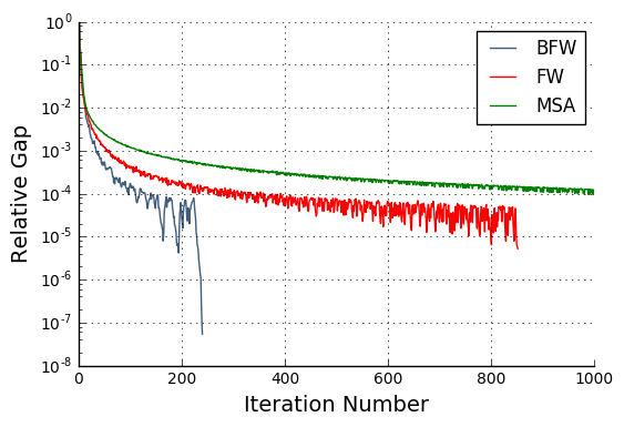
To give the reader a sense of how much faster the FW family are, let us take the example of a typical Australian road network, namely the inner Brisbane area during the morning peak (7 am to 9 am). In the following figure, we show the relative gap, which is a widely used measure of convergence, as a function of the number of iterations.

A relative gap of 10^-4 is generally considered to be sufficient for link flow stability. As can be seen the green line corresponds to MSA takes approximately 1000 iterations to reach this level compared to approximately 250 and 150 for the more advanced algorithms. Because each iteration is approximately equal in terms of runtime, this means that we can achieve an almost 8 fold decrease in our model runtime without sacrificing our ability to converge to a stable solution.
In this particular model, the use of BFW instead of MSA leads to a reduction in our assignment runtime from 8 hours to just over 1 hour. That’s a huge time saving and means that our modelling teams can turn projects around quicker, or study more scenarios within a given timeframe. This development also gives our teams the ability to reach much higher convergence levels for applications that demand it. The BFW method (blue line) converged to 10-6 in just under two hours, a level of precision that is unattainable with MSA in realistic times.
Obviously, the total runtime of this algorithm is determined not just by how many iterations we run, but also by the duration of each individual iteration. In our next article, we’ll examine some of the ways in which we’ve improved the runtime of each individual iteration.


