Braess’s paradox and generated traffic – comparing apples and oranges
17 October 2022
Long considered an interesting but to me ultimately a whimsical mathematical construct, Braess’s paradox has increased in popularity as a reference for the folly of investing in roads, generally linking the paradox to the general finding that new roads generate new traffic.
The networks used in Braess’s paradox – from Nagurney & Nagurney (2022)
Personally, as an equilibrium modeller, I welcome the increased prominence of Braess’s paradox – it is a good introduction to the concept of equilibrium, the difference between user equilibrium and system optimum route choice, and what is possible if through planning, pricing we can move from selfish to cooperative behaviour. By the way, the difference between these two traffic states is sometimes called the price of anarchy (see O’Hare, Connors and Watling (2016) for a good description).
But Braess’s paradox is not responsible for, or even a reasonable explanation of induced demand, generated traffic, and therefore it is time to set the record straight.
The paradox was first described in a German paper by Dietrich Braess in 1968 and, according to the very accessible and fascinating description by Nagurney and Nagurney (2022), lay undiscovered by the English reading public till it was translated by John Murdoch in 1970.
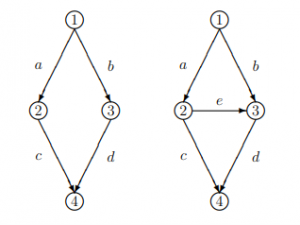
To explain the paradox, it is worth copying the simple network that Braess used (borrowed here from Nagurney and Nagurney, 2022, and illustrated at the top of this article)
The original network (left) consists of two routes 1-2-4 using links a and c and route 1-3-4 using links b and d; in the after situation (right) a new one-way link e is introduced enabling a third route 1-2-3-4 that uses links a, e and d.
The cost functions for all five links are as follows:

It is worthwhile understanding what these functions imply:
- Links a and c are short, direct routes but with very low capacity (no fixed costs but high marginal costs) – think narrow city centre roads
- Links b and d are high-capacity routes but quite a bit longer (fixed costs of 50 units, but with much lower marginal costs than links a and c) – think wide dual carriageway bypasses
- Link e is relatively short with similar capacity as links b and d, think of a wide bridge, for example
It is important to note that link e is one way, connecting the two narrow roads with a high-capacity bridge. Also, the cost functions of links a and d are such that at free flow they cost 0 units to traverse, whereas then the costs of links b and d are already 50 units. Only at link flows exceeding 6 vehicles per hour (vph) the costs of links b and c (60 units) are greater than those of links b and d (56 units).
In the before case, any demand between origin 1 and destination 4 will generate a 50/50 split between the two feasible routes. In Braess’s example a total demand of 6 vph is assumed and this demand distributes itself in a user equilibrium evenly across the two routes, 3 vph per route, at a cost of 30+53=83 units (you can easily check this yourself).
With link e introduced, the alternative 1-2-3-4 offers a new lower cost alternative at the original flow distribution (30+30+10=70 units) compared to the existing cost of 83 units, and the equilibrium is disturbed. Remember, at equilibrium all used routes are of equal length and shorter than any unused routes. Traffic re-routes and for the example of a total demand of 6 vph a new equilibrium is established with 2 vehicles using each of routes 1-2-4, 1-3-4 and 1-2-3-4. Every traveller now experiences a cost of 92 units (again, you can check this out for yourself). This is a deterioration in the costs from the situation before the bridge was built; hence the paradox that adding more capacity leads to longer travel times. Note that the original route pattern is still feasible, but that this could not be an equilibrium as in that situation there exists an unused alternative with a lower cost – in this case the price of anarchy is 92-83=9 units.
How is this possible? It’s because there are three specifically fabricated conditions:
1. the one-way bridge is built so that it connects the two narrow roads that previously were not connected. Would that happen in reality? Let’s look at the alternative that the bridge is built in the other direction, connecting the two high-capacity links. The new connection now has a cost at the originally established equilibrium of 53+53+10=106 units, so is not a feasible alternative for this demand level: the equilibrium will not be disturbed.
2. the cost curves (speed-flow curves) are unlikely to reflect a reasonable reality (the marginal costs of links a and d being ten times these of links b and c). In practice I would expect these to differ perhaps by a factor 2 or 3, not 10. The fixed costs of links b and d are also very high.
3. the travel demand is neither so low that using the bridge is attractive even after the equilibrium has been re-established, nor so high that the high marginal costs of links b and c would become prohibitive for the new route that includes both of them. Nagurney and Nagurney refer to Pas and Principio (1997) who calculated that the paradox only exists for demand between 2.58 and 8.89, a very narrow band indeed and certainly not at the very high values at which you would expect serious congestion and the likelihood of induced demand. You can check yourself that at a demand flow of 2 the new route 1-2-3-4 is the most attractive one for all travellers, at a cost of 20+20+12=52, whereas the original split across routes 1-2-4 and 1-3-4 gives a cost of 10+51=61 units – in other words, a benefit results from building the bridge. For a demand of 9 the original routes have a cost of 45+54.5=99.5, whereas the new route has a cost of 45+45+14.5=104.5, so is not an attractive alternative for switching).
This is why using the Braess paradox to explain induced demand is so unhelpful.
1. In reality, generated traffic occurs at high congestion levels, when latent demand tends to fill in newly released capacity. Build it and they will come. The Braess paradox in his original example only occurs at intermediate levels of congestion.
2. The real mechanism of induced demand is very different to what Braess illustrated. In his case re-routing of a fixed demand matrix takes place to satisfy equilibrium requirements in a carefully constructed example under very specific conditions. Generated traffic is the result of a much wider host of responses to increased road capacity in the real world, such as trip retiming back to the peak, strategic rerouting from outside the analysed area, mode shifts from public and active transport alternatives and re-distribution to more accessible destinations, all reflected in a variable demand matrix.
3. And the phenomenon of disappearing or evaporating traffic can be explained in much the same way.
Braess’s paradox is about route choice and equilibrium modelling. Does this mean that Braess’ paradox is not of any use? Not necessarily. It illustrates nicely that in any equilibrium context selfish optimisation may lead to suboptimal outcomes in which everyone loses; and that intervention may be required to stop that from happening, supporting the case for marginal cost road pricing, for instance.
For me, generated or disappearing traffic is much more easily explained by economic arguments rather than clever maths: make something cheaper and people will buy or use it more, increase the price and they will find alternatives. Best leave Braess’s paradox in textbooks for Master’s courses in transport.
References
Braess, D., 1968. Ueber ein Paradoxon aus der Verkehrsplanung. Unternehmensforschung 12, 258-268 (https://homepage.ruhr-uni-bochum.de/dietrich.braess/paradox.pdf)
Murchland J.D., 1970. Braess’s Paradox of Traffic Flow. Transportation Research 4, 391-394.
Nagurney, A. and Nagurney, L.S., 2022. The Braess Paradox, Invited Chapter for International Encyclopedia of Transportation, R. Vickerman, Editor, Elsevier (https://supernet.isenberg.umass.edu/articles/braess-encyc.pdf)
O’Hare, S., Connors, R.D. and Watling, D.P., 2016. Mechanisms that Govern how the Price of Anarchy varies with Travel Demand. Transportation Research Part B: Methodological, 84. pp. 55-80. https://eprints.whiterose.ac.uk/92812/8/TRB-OHareConnorsWatling.pdf
Pas, E.I. and Principio, S.L., 1997. Braess’ Paradox: Some New Insights. Transportation Research B 31(3), 265-276.